Supported Features
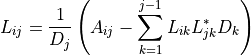
Introduction
Conventions
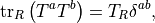
This section summarizes the main formulae that are used for implementing the HMC for dynamical Wilson fermions in higher representations. The Dirac operator is constructed following [LSSW96], but using Hermitian generators

For the fundamental representation, the normalization of the generators is such that:

For a generic representation  , we define:
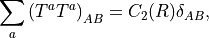
which implies
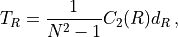
where  is the dimension of the representation . The relevant group factors may be computed from the Young tableaux of the representation of
  using
using
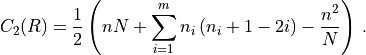
Here  is the number of boxes in the diagram,
  ranges over the rows of the Young tableau,
  is the number of rows, and
  is the number of boxes in the -th row.
R |
|
|
|
|---|---|---|---|
fundamental (fund) |
|
|
|
adjoint (adj) |
|
|
|
two-index symmetric (2S) |
|
|
|
two-index antisymmetric (2AS) |
|
|
|


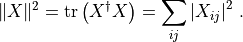
A generic element of the algebra is written as  and the
scalar product of two elements of the algebra is defined as
and the
scalar product of two elements of the algebra is defined as

 matrices
We use the chiral representation for the Dirac matrices where
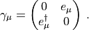
Then  are
are  matrices given by
  ,
,  corresponding to
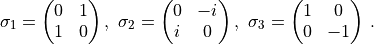
Finally
The Dirac operator
The massless Dirac operator is written as in [LSSW96]
with


and therefore the action of the massive Dirac operator yields
(1)
where  are the link variables in the representation .
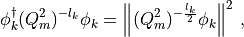
Rescaling the fermion fields by  , we can write the fermionic action as:
where
![D_m(x,y) = \delta_{x,y} - \frac{\kappa}{2}
\left[(1-\gamma_\mu) U^R(x,\mu) \delta_{y,x+\mu} +
(1+\gamma_\mu) U^R(x-\mu,\mu)^\dagger \delta_{y,x-\mu} \right],](../_images/math/08b9391b6faf0c273ac33df29de7fa1c74652697.png)
and the Hermitian Dirac operator is obtained as
(2)
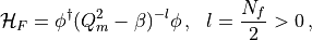
The fermionic determinant in the path integral can be represented by introducing complex pseudofermionic fields:
Force for the HMC molecular dynamics
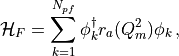
The HMC Hamiltonian is given by
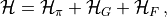
where
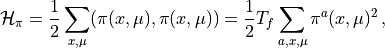
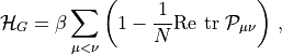
(3)
and we have introduced for each link variable a conjugate momentum in the algebra of the gauge group, defined as
In the expression of  we omitted the sum over position, spin
and color indices and we have also introduced an arbitrary shift
we omitted the sum over position, spin
and color indices and we have also introduced an arbitrary shift  for the matrix
  , as this will be useful in the discussion for the
RHMC algorithm.
, as this will be useful in the discussion for the
RHMC algorithm.
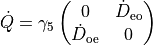
The equations of motion for the link variables are given by
The notation  indicates the derivative with respect to the molecular dynamics time.
We obtain the equations of motion for the momenta from the requirement that the Hamiltonian  is a conserved quantity
(4)
For the first two derivatives we have
(5)
(6)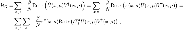
where  is the sum of the staples around the link
  .
.
The computation of the fermionic force goes as follows. We only consider
the case  since this is the only case relevant both for the HMC
algorithm and the RHMC algorithm (see below). We have
since this is the only case relevant both for the HMC
algorithm and the RHMC algorithm (see below). We have
(7)
Defining
(8)

and using the fact that the matrix  is Hermitian, we can rewrite (7) as
(9)
Inserting the explicit form of  , eqs. (2) and (1) into eq. (9) we obtain
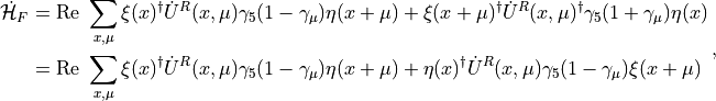
where the sum over spin and color indices is intended and we made explicit the fact that the whole expression is real. Further
(10)
Notice, that since we define  , the
, the
 in the above equation are the same as those appearing in
the expressions for
in the above equation are the same as those appearing in
the expressions for  . Using eq. (10) in the
expression for
. Using eq. (10) in the
expression for  we find
(11)![\begin{aligned}
\dot{\mathcal{H}}_F = \sum_{x,\mu} \sum_a \pi^a(x,\mu) & \mathrm{Re\ Tr\ } \left[ iT^a_R U^R(x,\mu) \gamma_5 (1-\gamma_\mu) \right.
\left. \left\{ \eta(x+\mu)\otimes\xi(x)^\dagger + \xi(x+\mu)\otimes\eta(x)^\dagger \right\} \right] \, .\end{aligned}](../_images/math/a2aba40dfd02f4d826f7c7ec7962dfe5d7876bf0.png)
Note that capitalized  indicates the trace over both color and spin indices as opposed to the lower case
  , which is the trace over color only.
Inserting eqs. (5), (6) into eq. (4) we obtain the equations of motion for the momenta
(12)
(13)![\dot\pi^a_G(x,\mu) &= \frac{\beta}{N} \frac{1}{T_f} \mathrm{Re\ tr\ } \left[ i T^a_f U(x,\mu) V^\dagger(x,\mu) \right] \, ,](../_images/math/e72f0bd9e1648d852bebd60b8e6a84612f3b58e2.png)
(14)![\dot\pi^a_F(x,\mu) &=-\frac{1}{T_f} \mathrm{Re\ Tr\ } \left[ iT^a_R U^R(x,\mu) \gamma_5 (1-\gamma_\mu) \left\{ \eta(x+\mu)\otimes\xi(x)^\dagger + \xi(x+\mu)\otimes\eta(x)^\dagger \right\} \right]\, .](../_images/math/9c735587484097aef533096d8672f3ecec8a989d.png)
For sake of convenience we introduce the following projectors  over the algebra in the representation
![P^a_R ( F ) = - \frac{1}{T_R} \mathrm{Re\ tr\ } \left[ i T^a_R F \right] \, ,](../_images/math/d6bdca9091535fc01971a46369f2fec464f6b89a.png)
which can be used to rewrite eqs (13) and (14) in a more compact form:
(15)![\begin{aligned}
\dot\pi^a_G(x,\mu) &= - \frac{\beta}{N} P^a_f \left( U(x,\mu) V^\dagger(x,\mu) \right) \, ,\\
\dot\pi^a_F(x,\mu) &= \frac{T_R}{T_f} P^a_R \left( U^R(x,\mu) \mathrm{tr_{spin}} \left[ \gamma_5 (1-\gamma_\mu) \left\{ \eta(x+\mu)\otimes\xi(x)^\dagger + \xi(x+\mu)\otimes\eta(x)^\dagger \right\} \right] \right)\, . \end{aligned}](../_images/math/ed3e012cf5b41f512dafa3d3b166144075fc2dd3.png)
Checks of the MD force
The formulae derived in the previous section can be checked against two
known examples. The first, and almost trivial, check is obtained by
assuming that the representation is again the fundamental
representation. The well-known expression for the MD force for the usual
HMC is then recovered.
The second case that has already been studied in the literature is the
case of fermions in the adjoint representation of the gauge group
SU( ) [DG96]. We agree with eq. (16) in
[DG96], provided that we exchange the indices
) [DG96]. We agree with eq. (16) in
[DG96], provided that we exchange the indices  and
and
 in that formula.
HMC Algorithm
Given the action  of a system of bosonic fields
  , our
goal is to generate a Markov process with fixed probability distribution
, our
goal is to generate a Markov process with fixed probability distribution
![P_S(\phi) = Z^{-1} \exp[-S(\phi)]](../_images/math/0e5bbf284bbc5585b5f9988286e0b633575afcd7.png) . A sufficient condition to have such a
Markov process is that it is ergodic and it satifies detailed balance:
. A sufficient condition to have such a
Markov process is that it is ergodic and it satifies detailed balance:

We define  with the following three-step
process:
with the following three-step
process:
We expand the configuration space with additional fields, the momenta
 randomly chosen with probability
  such
that
such
that  – usually one takes
![P_k(\pi)\propto \exp[-\pi^2/2]](../_images/math/e8c808298c3c8974e84d360281921d7c15245dce.png) ;
;In the extended configuration space
 , we generate a new
configuration
, we generate a new
configuration  with probability
 such that
(reversibility condition)
We accept the new configuration
 with probability
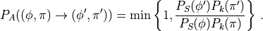
It is easy to see that the resulting probability

satisfies detailed balance. Care must be taken to ensure ergodicity.
As already stated, the distribution is generally taken to be
Gaussian (this should also guarantee ergodicity). The process  is
instead identified with the Hamiltonian flow of a yet unspecified
Hamiltonian
is
instead identified with the Hamiltonian flow of a yet unspecified
Hamiltonian  in the phase space
  (giving to the
meaning of “momenta”). The time reversal symmetry of classical dynamics
equation of motion guarantees the reversibility condition. The resulting
probability is then a delta function (the process is completely
deterministic). Numerical integration to a given accuracy will result in
a broader distribution and care must be taken to guarantee the
reversibility condition in this case. Since we want a high acceptance
rate (low correlation among the configurations), we must carefully
choose the Hamiltonian . One simple way is to take
(giving to the
meaning of “momenta”). The time reversal symmetry of classical dynamics
equation of motion guarantees the reversibility condition. The resulting
probability is then a delta function (the process is completely
deterministic). Numerical integration to a given accuracy will result in
a broader distribution and care must be taken to guarantee the
reversibility condition in this case. Since we want a high acceptance
rate (low correlation among the configurations), we must carefully
choose the Hamiltonian . One simple way is to take  to be
Gaussian and define
to be
Gaussian and define
![H(\pi,\phi)=-\ln [P_k(\pi) P_S(\phi)] = \pi^2/2 + S(\phi)](../_images/math/31f2060a8594a1133b8ad636d14cf3264794d51e.png)
(omitting irrelevant constants). If is exactly conserved by the process
then the acceptance probability is 1.
When fermionic degrees of freedom are present in the action  , we can
first integrate them out, resulting in a non-local bosonic action and
then apply the above scheme. In practice, to deal with a non-local
action is not convenient from a numerical point a view and stochastic
estimates are used.
, we can
first integrate them out, resulting in a non-local bosonic action and
then apply the above scheme. In practice, to deal with a non-local
action is not convenient from a numerical point a view and stochastic
estimates are used.
Consider a quadratic fermionic term in the action
with a generic interaction matrix  depending on the bosonic fields . The contribution of this term to the partition function is
![\int d\bar\psi d\psi \exp [ -S(\bar\psi,\psi)] = \mathrm{det}[M(\phi)]\, .](../_images/math/61d4505abbac1926097f0f3e7210d4b3b9cdf0ff.png)
Assuming that the matrix is positive definite, we can rewrite
![\mathrm{det}[M]=\int d\bar\eta d\eta \exp[ \bar\eta (M)^{-1} \eta ]\, ,](../_images/math/186779216dd1c7eeda49a1efea3c8921edb3b8bf.png)
where  ,
, are two new complex bosonic fields, called
pseudofermions. This term can be taken into account generating random
pseudofermions , with the desired probability
distribution and keeping then fixed during the above HMC configuration
generation for the remaining bosonic fields .
are two new complex bosonic fields, called
pseudofermions. This term can be taken into account generating random
pseudofermions , with the desired probability
distribution and keeping then fixed during the above HMC configuration
generation for the remaining bosonic fields .
RHMC formulation
The fermionic part of the HMC Hamiltonian, for  degenerate quarks
and
degenerate quarks
and  pseudofermions, can be written as:
(16)
and  . For the sake of simplicity we will set all the
  to be
equal:
to be
equal:

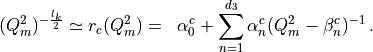
In the RHMC algorithm [CdFK06] rational approximations are used
whenever we need to take some fractional power of the positive definite
fermion matrix .
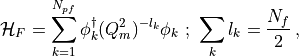
In this implementation we use three different rational approximations. The first one is used to approximate eq. (16). Here, we need only one approximation because all are equal yielding
(17)
Using the formulae derived in the previous sections, it is easy to write the force corresponding to eq. (17). In fact, eq. (17) is nothing but a sum of terms of the form eq. (17) once we put ,  . The RHMC force will be then given by a sum over
  of terms given by
eq. (15) multiplied by a factor
of terms given by
eq. (15) multiplied by a factor  . Notice that since , to compute as in eq. (8) a simple shifted inversion is required.
The second rational approximation is required in the heat bath update of
pseudofermions. In order to generate pseudofermions distributed as in
eq. (16), a simple two-step process is used. For each pseudofermion we first generate a gaussian distributed field 
![P(\tilde\phi_k)\propto \exp [ -\tilde\phi_k^\dagger \tilde\phi_k ] \, ,](../_images/math/bd524912bec5657d1368529f5e73b5c5d713ff16.png)
and then set
making use of the fact that  is Hermitian (notice the plus sign
in the exponent). The RHMC algorithm uses a rational approximation to
compute the above quantities. Again we need only one approximation since
all are equal.
is Hermitian (notice the plus sign
in the exponent). The RHMC algorithm uses a rational approximation to
compute the above quantities. Again we need only one approximation since
all are equal.
The third rational approximation is used in the code for the Metropolis test. Starting from eq. (16) for each pseudofermion we can rewrite:
where we used the property that is Hermitian. The rational
approximation needed in this case is:
Notice that if  the coefficients for the two approximations
 and
and  can each be obtained from the other.
In order to compute the coefficients  ,
,  appearing in
the rational approximations the Remez algorithm is needed. In this
implementation we do not compute those coefficients “on the fly”, but
rather we use a precomputation step to generate a table of coefficients
from which we pick up the right values when needed. The generation of
this table goes as follows:
appearing in
the rational approximations the Remez algorithm is needed. In this
implementation we do not compute those coefficients “on the fly”, but
rather we use a precomputation step to generate a table of coefficients
from which we pick up the right values when needed. The generation of
this table goes as follows:
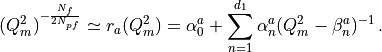
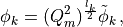
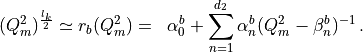
First note that we need to compute rational approximations for a
function  of the form
  and the approximation must be
accurate over the spectral range of the operator . To simplify
the computation of the table we note that the following proposition
holds: if is a homogeneous function of degree
and the approximation must be
accurate over the spectral range of the operator . To simplify
the computation of the table we note that the following proposition
holds: if is a homogeneous function of degree  and
and  is
an optimal (in the sense of relative error) rational approximation to
over the interval
is
an optimal (in the sense of relative error) rational approximation to
over the interval ![[\epsilon,\mathrm{h}]](../_images/math/9c8277859b5df3a542710c0419de55d76c8cdcf7.png) to a given accuracy
then
to a given accuracy
then  is an optimal rational approximation for the same
function and the same accuracy over the interval
is an optimal rational approximation for the same
function and the same accuracy over the interval
![[\epsilon/k,\mathrm{h}/k]](../_images/math/3496a88f27f5bc873b218f80d3e6ad8afa1b3ce5.png) . Notice that the coefficients of the
“rescaled” rational approximation are easily obtained from that of the
original approximation. A simple corollary is that, given a homogeneuos
function , we can divide the rational approximations with the same
accuracy in classes distinguished by the ratio
. Notice that the coefficients of the
“rescaled” rational approximation are easily obtained from that of the
original approximation. A simple corollary is that, given a homogeneuos
function , we can divide the rational approximations with the same
accuracy in classes distinguished by the ratio  ;
within each class the coefficients of the rational approximations are
easily related to each other, so that we only need to compute one
rational approximation in each class. This is what is done in our
implementation.
;
within each class the coefficients of the rational approximations are
easily related to each other, so that we only need to compute one
rational approximation in each class. This is what is done in our
implementation.
In detail: we generate a table containing the coefficients for the
rational approximations belonging in different classes distinguished by
the function which we want to approximate and the accuracy which
is required. We arbitrarily set  to a fixed value equal to the
absolute upper bound on the spectrum of the matrix . This choice
fixes the representative of each class, because the lower bound of the
approximation is now a function of .
to a fixed value equal to the
absolute upper bound on the spectrum of the matrix . This choice
fixes the representative of each class, because the lower bound of the
approximation is now a function of .
At run-time this table is used to generate optimal rational
approximations rescaling the precomputed coefficients to the desired
interval containing the spectrum of the matrix . This interval is
obtained by computing the maximum and minimum eigenvalue of on
each configuration when needed. In our code we update this interval only
before the metropolis test, while we keep it fixed during the molecular dynamics.
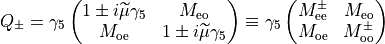
Even-Odd preconditioning
It is a very well know fact that the time spend for a simulation with
dynamical fermions is dominated by the time required for the inversions
of the Dirac operator. The convergence of such inversions can be
improved using appropriate preconditioning. The idea is to rewrite the
fermionic determinant as a determinant (or product of determinants) of
better conditioned matrix (matrices) than the original Dirac operator.
For the non-improved Wilson action this can be easily done using the
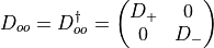
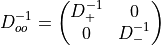
even-odd preconditioning. We start rewriting the Dirac operator  as a block matrix:
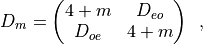
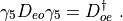
where each block has a dimension half that of the original Dirac matrix. The diagonal blocks connecting sites with the same parity are proportional to the identity matrix, while off-diagonal blocks connect sites with opposite parity. We have (since is  -hermitian):
The determinant of the Dirac matrix can be rewritten as:

using the well known formula for the determinant of a block matrix.
Since the determinant of and of  are the same the latter
can be used in numerical simulations. Note that the even-odd
preconditioned matrix only connects sites with the same parity thus it
have only half of the size of the original Dirac matrix and as it
is -Hermitian. We define as before the Hermitian matrix
are the same the latter
can be used in numerical simulations. Note that the even-odd
preconditioned matrix only connects sites with the same parity thus it
have only half of the size of the original Dirac matrix and as it
is -Hermitian. We define as before the Hermitian matrix
 , which will be used in practice.
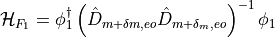
The formulation of the HMC algorithm does not change and the only difference is that pseudofermionic fields are now only defined on half of the lattice sites, conventionally the even sites in what follows. We now give the explicit expression for the fermionic force for the preconditioned system described by the Hamiltonian:
where as before we are assuming  or a rational approximation of
the actual fractional power function, and where we made explicit that
or a rational approximation of
the actual fractional power function, and where we made explicit that
 is only defined on even sites. Eq. (9) is unchanged:
(18)
where as before we have defined:


The explicit form of  must be used at this point. We have:
(19)
Defining


and inserting eq. (19) into eq. (18) we find:
(20)![\begin{aligned}
\dot{\mathcal{H}}_F = - \sum_{\mu,x\in \mathrm{even}} {\rm Tr}_{x,\mu} \left[ \sigma_o(x+\mu)\otimes\xi_e(x)^\dagger + \rho_o(x+\mu)\otimes\eta_e(x)^\dagger \right] \\
- \sum_{\mu,x\in \mathrm{odd}} {\rm Tr}_{x,\mu} \left[ \xi_e(x+\mu)\otimes\sigma_o(x)^\dagger + \eta_e(x+\mu)\otimes\rho_o(x)^\dagger \right] \end{aligned}](../_images/math/56ad62b9fea6a781eda6e8ea1e41b801401083ba.png)
employing the shorthand notation:
![{\rm Tr}_{x,\mu} \left[ \Phi \right] \equiv \mathrm{Re\ Tr\ } \left[ \dot U^R(x,\mu) \gamma_5 (1-\gamma_\mu) \Phi \right]\,\, .](../_images/math/66133dc69d71f45e8500741e42894646129a8f8f.png)
From eq. (20) it is clear that the fermionic force has a different expression on sites of different parities. Proceeding as before we arrive at the final
expressions. For  :
:
![\dot\pi^a_F(x,\mu) &= - \frac{T_R}{T_f} P^a_R \left( U^R(x,\mu) \mathrm{tr_{spin}} \left[ \gamma_5 (1-\gamma_\mu) \left\{ \sigma_o(x+\mu)\otimes\xi_e(x)^\dagger + \rho_o(x+\mu)\otimes\eta_e(x)^\dagger \right\} \right] \right)\, ,](../_images/math/dfd7245ebc38934933f7f3b1b2d15a5bf8b13d24.png)
while for  :
:
![\begin{aligned}
\dot\pi^a_F(x,\mu) &= - \frac{T_R}{T_f} P^a_R \left( U^R(x,\mu) \mathrm{tr_{spin}} \left[ \gamma_5 (1-\gamma_\mu) \left\{\xi_e(x+\mu)\otimes\sigma_o(x)^\dagger + \eta_e(x+\mu)\otimes\rho_o(x)^\dagger \right\} \right] \right)\, .\end{aligned}](../_images/math/5af89c53100372457d1bcb4f970379eedbb7d384.png)
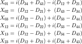
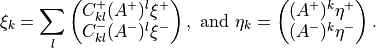
Two-point functions
This is a summary of the formulae used for the mesonic two-point
functions. Let  and
and  be two generic matrices in the Clifford
algebra. Then we define the two-point function
be two generic matrices in the Clifford
algebra. Then we define the two-point function
Performing the Wick contractions yields
![\langle \bar\psi({\bf x},t) \Gamma\psi({\bf x},t) \bar\psi(0) \Gamma^\prime \psi(0) \rangle =&- \mathrm{tr} \left[ \Gamma S(x-y) \Gamma^\prime S(y-x) \right]
= - \mathrm{tr} \left[ \Gamma S(x-y) \Gamma^\prime \gamma_5 S^\dagger(x-y) \gamma_5 \right]\,.](../_images/math/862a8290a862fd1a91f69e801c7ec741d18d7c21.png)
In practice we invert the Hemitian Dirac operator  by solving the equation:

where  is a collective index for colour and spin, and
 ,
,  are the position of the source for the inverter. Using the field that we obtain from the inverter, the correlator
above becomes:
are the position of the source for the inverter. Using the field that we obtain from the inverter, the correlator
above becomes:

where  , and
, and  .
.
Hasenbusch acceleration
Let us summarize the Hasenbusch trick (for two flavours)
where  is the hermitian Dirac operator. After integration over the pseudofermions it gives the determinant:
The Hasenbusch trick can be rewritten in the following form :
Where  can be chosen arbitrarily as long as the determinant is
well defined. We discuss in the next subsections various choices of
.
can be chosen arbitrarily as long as the determinant is
well defined. We discuss in the next subsections various choices of
.
In any case the two term can be evaluated independently, and we have:

This can be combined with even-odd preconditioning.
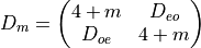
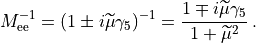
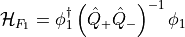
Wilson Mass Shift
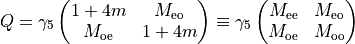
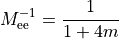
Assume

Note that, as written in a comment in the code, 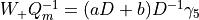 .
.
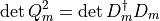
Then

The force can then be computed :
![\begin{aligned}
\dot{\mathcal{H}_{F_2}} =& - \delta_m \phi_2^\dagger \left[ \left( \gamma_5 + \delta_m Q^{-1}
\right) \dot{Q^{-1}} + \dot{Q^{-1}} \left( \gamma_5 + \delta_m Q^{-1}
\right) \right] \phi_2 \\
=& - \delta_m \phi_2^\dagger \left[ \left( \gamma_5 + \delta_m
Q^{-1}\right) Q_m^{-1} \dot{Q} Q_m^{-1} \right]\phi_2 + \rm{h.c}
\end{aligned}](../_images/math/82414b7d95ecc3046b05b4f37247fe0eec20af89.png)
Note that the equation as now the standard form of the forces for the HMC algorithm provided that:

From which we deduce

Which matches one comment in the the force_hmc.c file.
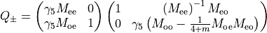
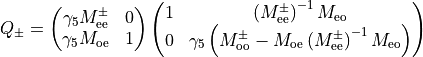
Even-Odd Preconditioning
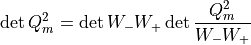
Writing
The determinant in the 2 flavour case can be written as follows:

Note that  can be computed:
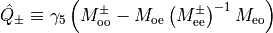
Now we can conveniently rewrite
From the last equation we deduce that:

Note that the first determinant is a constant that could be computed.
In the following we will denote

where  is defined on the odd sites of the lattice.
Now defining


We thus have
and

Note that as in the non-even-odd case this can be rewritten as:

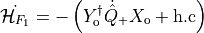
Twisted-Mass Shift
Assume

Note that 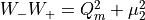 and that
  .
.
Instead of dealing with  , we consider the slightly more general case where the
determinant to evaluate is
, we consider the slightly more general case where the
determinant to evaluate is
![\begin{aligned}
\det{ (Q_m + i \mu_1) (W_-
W_+)^{-1} (Q_m - i \mu_1)}\propto&\int D\phi_2 D\phi_2^\dagger e^{-\phi^\dagger_2 \Big(Q_+ (W_-
W_+)^{-1} Q_- \Big)^{-1}\phi_2 }\big] \\
=& \int D\phi_2 D\phi_2^\dagger e^{-\phi_2Q_-^{-1} W_- W_+
Q_+^{-1} \phi_2 }\end{aligned}](../_images/math/4035bc4250250a5c336f3aedabc385fa0d3ba2b7.png)
The following formulae can then be used for the case of several Hasenbusch masses. The case of the determinant 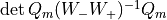 can be recovered by setting
  in the following equations.
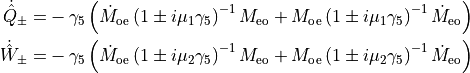
We have:
The force can then be computed: (global sign and factor have to be
checked)
![\begin{aligned}
\dot{\mathcal{H}_{F_2}} =& i(\mu_2-\mu_1) \phi_2^{\dagger} \Big[ ( 1 - i(\mu_2 - \mu_1)
(Q_m - i \mu_1)^{-1}) \dot{(Q_m+i\mu_1)^{-1}}
- \dot{(Q_m - i \mu_1)^{-1}} (1+ i (\mu_2 - \mu_1) (Q_m+i \mu_1)^{-1})\Big] \phi_2 \\
=& i(\mu_2-\mu_1) \phi_2^{\dagger} \left[ ( 1 - i(\mu_2 - \mu_1)
(Q_m - i\mu_1)^{-1}) ( Q_m+i\mu_1)^{-1} \dot{Q_m} (Q_m+i\mu_1)^{-1}
\right] \phi_2 +\rm{h.c}\end{aligned}](../_images/math/0e8eba36417968806dca81e9dece73965dc24605.png)
with

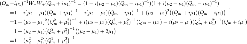
From this we deduce
Note that in the particular case where ,

Which leads to

Note also that the forces are explicitly proportional to  .
.
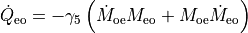
Even-Odd Preconditioning
Note that we have  .
.
can be computed as
Now we can conveniently rewrite
From the last equation we deduce that:

Note that the first determinant is a constant that could be computed. In the following we will denote
where  is defined on the odd sites of the lattice.
We thus have

and we thus get the following Hamiltonian:
The corresponding force then reads :

Now using that  , the previous equation can
be written:
, the previous equation can
be written:
with
where we have used that

Furthermore we have

Now noting that

we have
Choosing  ,
,
 ,
,  , and
, and  allows to
write
allows to
write

with
Here, we have used that  and
and
Determinant Ratio
We use that

We thus have to compute
![\begin{aligned}
\dot{\mathcal{H}_{F_2}} &=\, \phi_2^\dagger\big[ \delta \hat{W}_-
(\hat{Q}_+ \hat{Q}_-)^{-1} \hat{W}_+ + \hat{W}_-
(\hat{Q}_+ \hat{Q}_-)^{-1} \delta \hat{W}_+
+ \hat{W}_- \delta \hat{Q}_-^{-1} \hat{Q}_+^{-1} \hat{W}_+ +
\hat{W}_- \hat{Q}_-^{-1} \delta \hat{Q}_+^{-1} \hat{W}_+ \big] \phi_2 \\
&=\, \phi_2^\dagger\big[ \dot{\hat{W}}_-
(\hat{Q}_+ \hat{Q}_-)^{-1} \hat{W}_+ + \hat{W}_-
(\hat{Q}_+ \hat{Q}_-)^{-1} \delta \hat{W}_+
- \hat{W}_- \hat{Q}_-^{-1} \dot{\hat{Q}}_- \hat{Q}_-^{-1} \hat{Q}_+^{-1} \hat{W}_+ -
\hat{W}_- \hat{Q}_-^{-1} \hat{Q}_+^{-1} \dot{\hat{Q}}_+ \hat{Q}_+^{-1} \hat{W}_+ \big] \phi_2 \\\end{aligned}](../_images/math/8a9b5ce41004f86cb42cece7f2bb8d201705bb48.png)
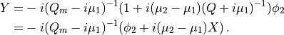
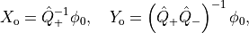
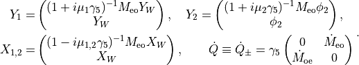
Now we introduce

such that

Now recalling that
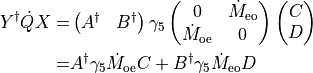
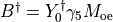
Now we can write the last expression in terms of  .
.
![\dot{\mathcal{H}_{F_2}} = Y_1^\dagger \dot{Q} X_1 + X_1^\dagger
\dot{Q} Y_1 - X_2^\dagger \dot{Q} Y_2 - Y_2^\dagger \dot{Q} X_2
= 2~ \rm{Re}\Big[ Y_1^\dagger \dot{Q} X_1 - Y_2^\dagger \dot{Q}
X_2 \Big]\,,](../_images/math/468646968d4847a4b27a1b22d2d3e0356f373e2e.png)
with
Twisted Wilson-Dirac Operator
Instead of applying the even-odd preconditioning to the twisted-mass operator we can use the Wilson-Dirac even-odd operator and do a different splitting.
We define

Now split the determinant
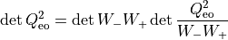
and choose
The corresponding Hamiltonian reads

Since the operators are now very similar to the non even-odd case, we can reuse some formulae. In particular, we can rewrite the Hamiltonian

From this we have the following forces:

Now we want to rewrite the last equation as a function of

where we have used that

Furthermore we have
noting that

and chosing ,  ,
,
 , and allows us to write:
with
We have used that  .
.
Similarly for the second Hamiltonian we get
which is exactly the force that appears in case of a pure Wilson-Dirac even-odd preconditioned operator up to a multiplicative factor.
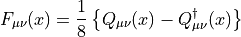
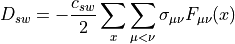
Clover Term
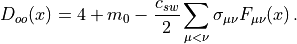
The clover term can be written as
(21)
with the (unconventional) definition of  given by
![\sigma_{\mu\nu} = \frac{1}{2}[\gamma_\mu,\gamma_\nu].](../_images/math/996f7ffff53e4d8cf73ca4027491755f9e3cb3aa.png)
With the Euclidean definition of the gamma matrices, satisfies
For the Hermitian Dirac operator  we can make the following replacement without affecting any of the calculations presented here
The field strength tensor is defined as
with
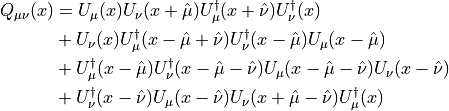
Because  we have
  .
For this reason we can change the sum over
.
For this reason we can change the sum over  in Eq. (21) to a sum over
  and a factor of two.
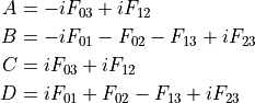
The quantity  is Hermitian and block diagonal.
It can be written as
is Hermitian and block diagonal.
It can be written as
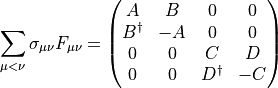
with the definitions
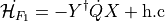
Pseudofermion Forces
For the forces we use the following short-hand notation for the derivative with respect to the link variables.

To calculate the pseudofermion forces let us write down the action as
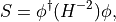
where  is the Hermitian Dirac operator.
When differentiating the action we obtain
is the Hermitian Dirac operator.
When differentiating the action we obtain
(22)
with the definitions

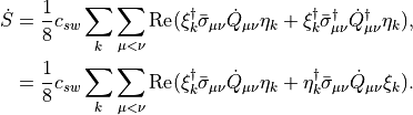
Forces
Here we will only consider the forces from the clover term and not the hopping term. The clover part of the Dirac operator is given by
(23)
When inserting Eq. (30) we obtain
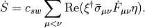
From the definition of  it follows that
This can in be written as
![\dot{S} = \frac{1}{8}c_{sw}\sum_{\mu<\nu} \mathrm{Re}~\mathrm{tr}\left[\dot{Q}_{\mu\nu}\left\{\bar{\sigma}_{\mu\nu}\eta(x)\otimes\xi^\dagger(x) + \bar{\sigma}_{\mu\nu}\xi(x)\otimes\eta^\dagger(x)\right\}\right]](../_images/math/7a418a0e9ed161ee803a7a90d73fc7bee3862b45.png)
In a short hand notation we need to calculate
(24)![\dot{S} = \frac{1}{8}c_{sw}\mathrm{Re}~\mathrm{tr}[\dot{Q}_{\mu\nu}(x)X_{\mu\nu}(x)]](../_images/math/84af680e1fd4629b3e615079d4b97920010a1969.png)
with

This matrix has the properties 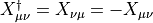 .
The expression for
.
The expression for  contains eight different terms (two from each of the four leafs).
The eight contributions to the force can be written as
contains eight different terms (two from each of the four leafs).
The eight contributions to the force can be written as
![\begin{aligned}
F_1(x) &=
\mathrm{Re}~\mathrm{tr}[\dot{U}_\mu(x)U_\nu(x+\hat{\mu})U_\mu^\dagger(x+\hat{\nu})U_\nu^\dagger(x)X_{\mu\nu}(x)] \\
F_2(x) &=
\mathrm{Re}~\mathrm{tr}[\dot{U}_\mu(x)U_\nu^\dagger(x+\hat{\mu}-\hat{\nu})U_\mu^\dagger(x-\hat{\nu})X_{\mu\nu}^\dagger(x-\hat{\nu})U_\nu(x-\hat{\nu})] \\
F_3(x) &=
\mathrm{Re}~\mathrm{tr}[\dot{U}_\mu(x)U_\nu^\dagger(x+\hat{\mu}-\hat{\nu})X_{\mu\nu}^\dagger(x+\hat{\mu}-\hat{\nu})U_\mu^\dagger(x-\hat{\nu})U_\nu(x-\hat{\nu})] \\
F_4(x) &=
\mathrm{Re}~\mathrm{tr}[\dot{U}_\mu(x)X_{\mu\nu}(x+\hat{\mu})U_\nu(x+\hat{\mu})U_\mu^\dagger(x+\hat{\nu})U_\nu^\dagger(x)] \\
F_5(x) &=
\mathrm{Re}~\mathrm{tr}[\dot{U}_\mu(x)X_{\mu\nu}^\dagger(x+\hat{\mu})U_\nu^\dagger(x+\hat{\mu}-\hat{\nu})U_\mu^\dagger(x-\hat{\nu})U_\nu(x-\hat{\nu})] \\
F_6(x) &=
\mathrm{Re}~\mathrm{tr}[\dot{U}_\mu(x)U_\nu(x+\hat{\mu})X_{\mu\nu}(x+\hat{\mu}+\hat{\nu})U_\mu^\dagger(x+\hat{\nu})U_\nu^\dagger(x)] \\
F_7(x) &=
\mathrm{Re}~\mathrm{tr}[\dot{U}_\mu(x)U_\nu(x+\hat{\mu})U_\mu^\dagger(x+\hat{\nu})X_{\mu\nu}(x+\hat{\nu})U_\nu^\dagger(x)] \\
F_8(x) &=
\mathrm{Re}~\mathrm{tr}[\dot{U}_\mu(x)U_\nu^\dagger(x+\hat{\mu}-\hat{\nu})U_\mu^\dagger(x-\hat{\nu})U_\nu(x-\hat{\nu})X_{\mu\nu}^\dagger(x)]
\end{aligned}](../_images/math/1ef01dbcfd9c04f71b7142a9be4c9c1ce7a0df39.png)
where each term should be multiplied by  .
The calculation can be done efficiently by noticing that several products and terms appear in multiple places.
Introduce the intermediate variables
.
The calculation can be done efficiently by noticing that several products and terms appear in multiple places.
Introduce the intermediate variables
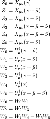
The total force can now be written as

This brings us down to a total of 15 matrix multiplications and 6 additions.
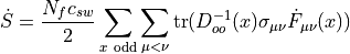
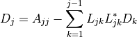
Logarithmic Forces
In the case of even-odd preconditioning the action of the small determinant  can be written as

The derivative is given by
![\dot{S} = -N_f\sum_{x~\mathrm{odd}}\mathrm{tr}\left[D_{oo}^{-1}(x)\dot{D}_{oo}(x)\right]](../_images/math/fbd9da9ded6df2d2bf3c80d5e126a279c3952ee5.png)
with  given by
Both the determinant and the inverse of can be calculated from an LDL decomposition.
If we insert the above definition we obtain
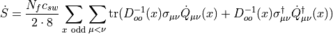
Since  is Hermitian we can write the result as two times the real part.
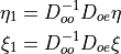
To simplify the result we define
is Hermitian we can write the result as two times the real part.
To simplify the result we define 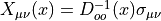 such that
![\dot{S} = \frac{N_fc_{sw}}{8}\sum_{x~\mathrm{odd}}\sum_{\mu<\nu}\mathrm{Re}~\mathrm{tr}[X_{\mu\nu}(x)\dot{Q}_{\mu\nu}(x)] \,.](../_images/math/429fd02b093246dd313c58fd0fb43821a5504ac3.png)
This is equivalent to eq. (33) except from the factor and the definition of  .
Notice that we still have the identity
.
Notice that we still have the identity  .
The sum over
.
The sum over  can be extended to all sites by setting
  to zero on the even sites.
To calculate the inverse we introduce the definitions:
to zero on the even sites.
To calculate the inverse we introduce the definitions:
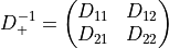
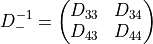
Because of hermiticity we know that  and
and  .
The six independent elements of can now be written as
.
The six independent elements of can now be written as
Even-odd Preconditioning
Method 1
We can write the determinant as

Use the notation
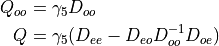
The action is

Forces for  -term
-term
The derivative is
![\dot{S}_1 = -2\mathrm{Re}\left[\phi_1^\dagger(Q_{oo}^{-2}Q_{oo}\dot{Q}_{oo}Q_{oo}^{-2})\phi_1\right]](../_images/math/23b7850b33c44ee9c36ae729a9163325e739767c.png)
and we can write it as
![\dot{S}_1 = -2\mathrm{Re}\left[\xi^\dagger\dot{Q}_{oo}\eta\right]](../_images/math/973ec419f00a9c90769b1480fc8227a6e437af15.png)
with

Forces for  -term
-term
The derivative is
![\dot{S}_2 = -2\mathrm{Re}\left[\phi_2^\dagger(Q^{-2}Q\dot{Q}Q^{-2})\phi_2\right]](../_images/math/b99a38bc8fe77c9a384ad6728575d848dcaed696.png)
and we can write it as
![\dot{S}_2 = -2\mathrm{Re}\left[\xi^\dagger\dot{Q}\eta\right]](../_images/math/08c828374c72ed1796aaca7c91d2cdbe66da0e9b.png)
with

The explicit expression for  is given by

and it can be written as

with
Method 2
The action of can also be expressed directly as the logarithm of the determinant.

This is the approach implemented in the code.
LDL factorization
With even-odd preconditioning we need to calculate the inverse when applying the dirac operator and when calculating the forces.
Because this matrix is Hermitian and block diagonal it can be inverted locally with an exact solver.
The most practical solver is via an LDL decomposition.

Sum over 
Sum over  .
.
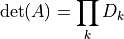
The determinant is given by
LDL Decomposition
Calculates the LDL decomposition  in-place.
After the decomposition, the lower triangular part of
in-place.
After the decomposition, the lower triangular part of  is
is  and the diagonal is
  .
.
do i=0, N-1
    do k=0, i-1
        A_ii = A_ii - L_ik * conj(L_ik) * A_kk
    enddo
    do j=i+1, N-1
        do k=0, i-1
	    A_ji = A_ji - A_jk * conj(L_ik) * A_kk
	enddo
	A_ji = A_ji/A_ii
    enddo
enddo
Forward substitution
Calculates  .
.
do i=0, N-1
    x_i = b_i
    do k=0, i-1
        x_i = x_i - A_ik * x_k
    enddo
enddo
Backward substitution with diagonal
Calculates  .
.
do i=N-1, 0
    x_i = x_i/A_ii
    do k=i+1, N-1
        x_i = x_i - conj(A_ki) * x_k
    enddo
enddo
Full inversion
This algorithm calculates the inverse  from the LDL decomposition.
Because the inverse is Hermitian we only calculate the lower triangular part.
from the LDL decomposition.
Because the inverse is Hermitian we only calculate the lower triangular part.
do i=0, N-1
    B_ii = 1
    do j=i, N-1
        do k=i, j-1
	    B_ji = L_jk * B_ki
	enddo
    enddo
    do j=N-1, i
        B_ji = B_ji/L_ii
	do k=j+1, N-1
	    B_ji = conj(L_kj) * B_ki
	enddo
    enddo
enddo
Exponential Clover Term
The exponential version of the clover term (including mass term) can be written as
(25)
where is again defined by
![\sigma_{\mu\nu} = \frac{1}{2}[\gamma_\mu,\gamma_\nu].](../_images/math/386dcdc65a5de5c41ffd4929a7c3a296bc8e86d1.png)
As for the clover term above, we can simplify the sum over  to a sum over
  and introduce a factor of two. We define
(26)
The quantity is Hermitian and block
diagonal. It can be written as
(27)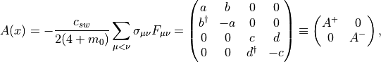
where  are
are  matrices in spin space and
  are
are  .
.
This formulation of  as a block matrix will be useful for the
exponentiation.
as a block matrix will be useful for the
exponentiation.
Evaluation of the operator
The evaluation of the exponential of can be split as:
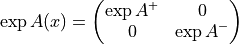
and so, the problem is reduced to the exponential of two
 matrices. The evaluation can be performed in
two ways.
matrices. The evaluation can be performed in
two ways.
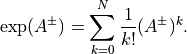
Using the Taylor expansion:
Using the Horner scheme:
(28)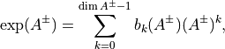
where  are computed recursively as follows. We start with

Then, the recursion proceeds:


(29)
where  represent the coefficients of the characteristic polynomial of the matrix
For instance, the characteristic polynomial of a  traceless matrix has the following coefficients:

Finally, the coefficients of eq. (28) are  .
.
The Horner scheme method is currently implemented only for  and
and
 with fundamental fermions.
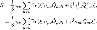
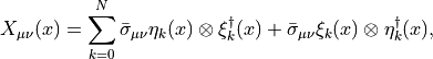
Pseudofermion Forces
For the forces we use the following shorthand notation for the derivative with respect to the link variables.

To calculate the pseudofermion forces let us write down the action as

where is the Hermitian Dirac operator. When differentiating the action we obtain
(30)
with the definitions

Forces
Here we will only consider the forces from the clover term. For the exponential version of the clover term, the implementation is very similar to the traditional clover term.
The clover part of the Dirac operator is given by
(31)
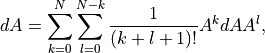
An optimized way of calculating the derivative is provided by the double Horner scheme. The basic idea is that the derivative of a matrix can be expressed as:
(32)
where the  coefficients depend on the matrix , similarly to
the ones eq. (28). They are calculated performing first the
iteration in eq.
coefficients depend on the matrix , similarly to
the ones eq. (28). They are calculated performing first the
iteration in eq. horner, and then repeating the iteration process on the result of the first iteration. For compactness, we shall omit the limits of the sum henceforth. When inserting eq. (31) in eq. (30), and using eq. (32) we obtain
with
From the definition of it follows that
This can in be written as
![\dot{S} = \frac{1}{8}c_{sw}\sum_{\mu<\nu} \mathrm{Re}~\mathrm{tr}\left[\dot{Q}_{\mu\nu} \sum_k\left\{\bar{\sigma}_{\mu\nu}\eta_k(x)\otimes\xi_k^\dagger(x) + \bar{\sigma}_{\mu\nu}\xi_k(x)\otimes\eta_k^\dagger(x)\right\}\right]](../_images/math/bc4c24150084d6a54936bd0cb9bcc1ef7c0cfd72.png)
As for the clover term above we need to calculate now
(33)![\dot{S} = \frac{1}{8}c_{sw}\mathrm{Re}~\mathrm{tr}[\dot{Q}_{\mu\nu}(x)X_{\mu\nu}(x)]](../_images/math/ab5a9125b19f40c1fd205fbce526ad73a7c9dc35.png)
now with

The total force can now be expressed as in the clover term above.
Even-odd Preconditioning
Even-odd preconditioning is particularly simple for the exponential case, since the force coming from the little determinant vanished. This can be seen because of the fact that:

and so it is a constant term in the action that does not contribute to the force.
Implementation of using Taylor Series
In the current version of the code, the Horner scheme is only implemented
for and with fundamental fermions. For other theories, a
less efficient, but more flexible, alternative is used. For this,
we use the Taylor series
with  sufficiently large. The implementation changes only in the definition of :
where now

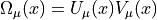
Stout smearing
The implementation follows [MP04] closely. We define the smeared links as
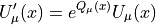
where  is an element of the Lie algebra, defined via the
projection
is an element of the Lie algebra, defined via the
projection
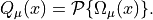
The projection operator is not unique, but the most common choice is
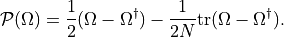
However, in a setup with mixed representations, it is convenient to use the following two-step procedure for the projection. This allows us to project matrices from different representations onto the generators of the fundamental representation.
![\begin{aligned} A_\mu^a(x) &= -\frac{1}{T_f}\mathrm{tr}[iT^a_R\Omega_\mu(x)] \\ Q_\mu(x) &= iT^a_F A_\mu^a(x)\end{aligned}](../_images/math/354ba794092f78543c71791fefcabd4e0b249516.png)
The matrix  is defined as

For the force calculation we use the chain rule.
The first derivative on the right-hand side is the usual force
 evaluated using the smeared links. The second term is
the derivative of the smeared links with respect to the fundamental
links. This can be written in the following way, because the derivative
of the action is surrounded by a trace.
evaluated using the smeared links. The second term is
the derivative of the smeared links with respect to the fundamental
links. This can be written in the following way, because the derivative
of the action is surrounded by a trace.
When using a Taylor expansion to define the exponential function, we can
use the following definition of  .
.

The derivative of the  matrix is the last missing piece. Define
 and consider

Here we have a sum over  . There are eight contributions to
the above derivative.
. There are eight contributions to
the above derivative.


This can be simplified because several products appear more than once
and we can use  to remove some of the
Hermitian conjugates. In the following we also assume that
to remove some of the
Hermitian conjugates. In the following we also assume that
 .
.


Here

This brings us down to 13 multiplications.